plot.pumping_test

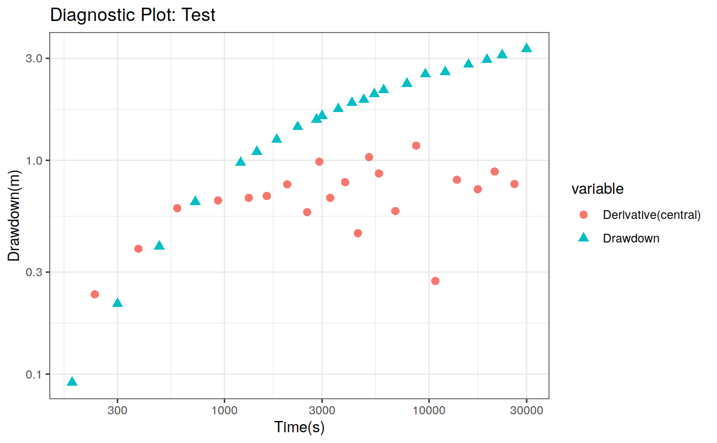
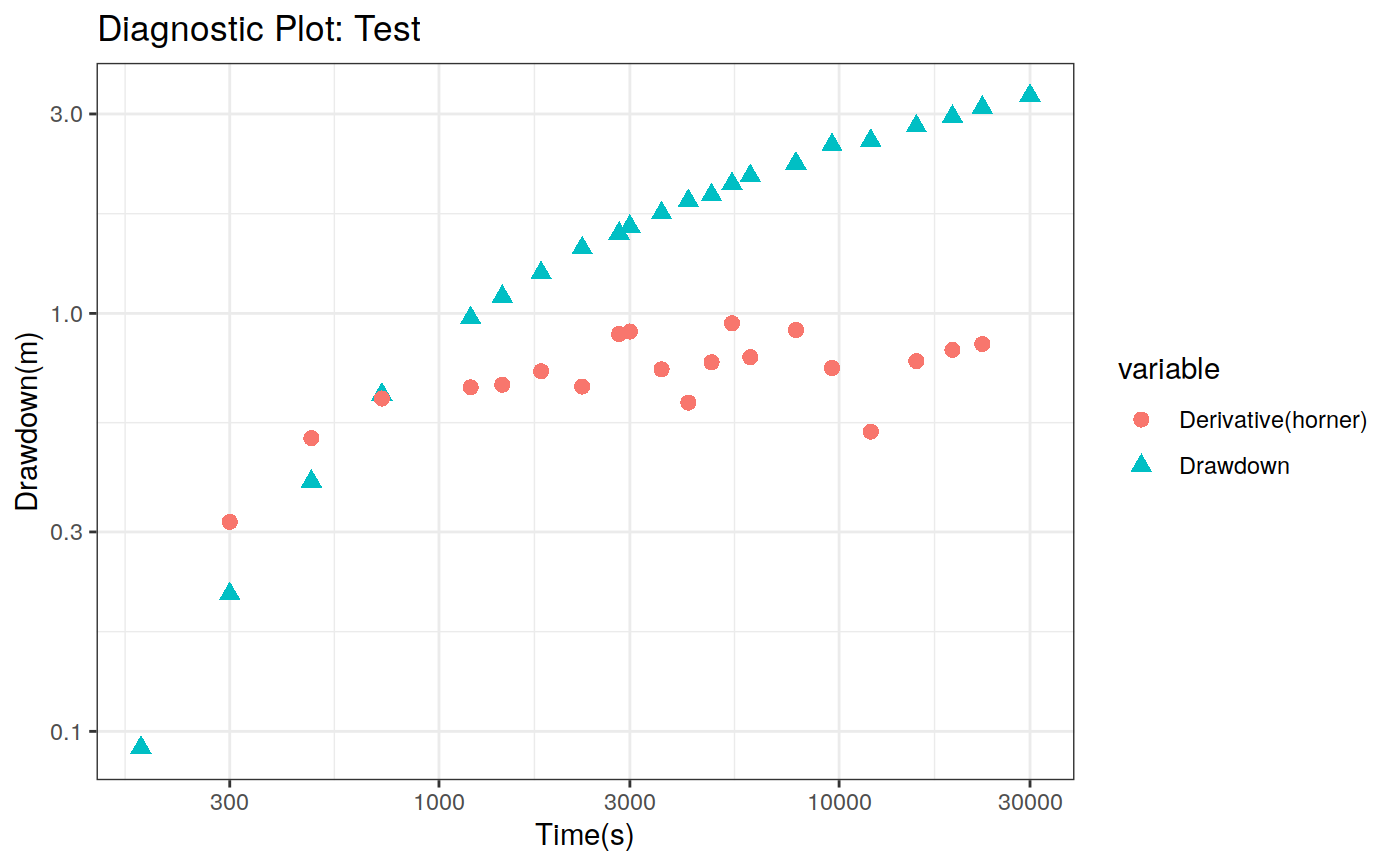
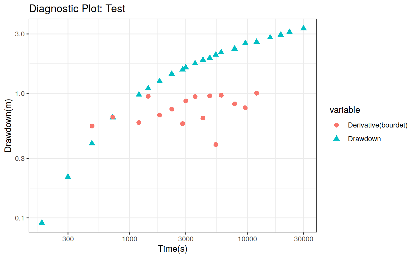
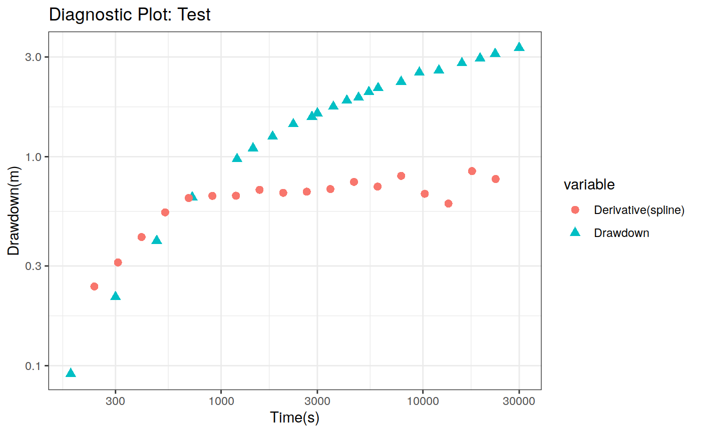
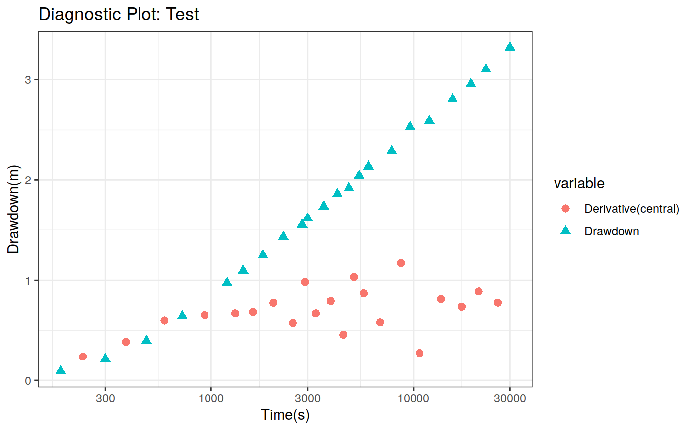
Function to plot the pumping test data. This function can create two different types of plots: diagnostic and estimation. The diagnostic plot includes the drawdown vs time plot and the derivative of drawdown with respect to the log of time. This derivative can help in the identification of the flow regime that occurred when the data was acquired.

# S3 method for pumping_test
plot(x, type = c("diagnostic", "estimation",
  "model.diagnostic", "uncert", "mcmc.trace", "mcmc.run_mean",
  "mcmc.compare", "mcmc.autocorr", "sample.influence"),
  dmethod = "central", d = 2, scale = "loglog", y.intersp = 0.5,
  slug = FALSE, legend = TRUE, results = FALSE, cex = 1, ...)

Arguments

x	A pumping_test object
type	Type of plot. Current options include diagnostic estimation model.diagnostic uncertainty mcmc.trace mcmc.run_mean mcmc.compare mcmc.autocorr sample.influence
dmethod	Method to calculate the derivative (central, horner, bourdet, spline)
d	Derivative parameter. If method is bourdet then d is a parameter to specify the number of lags in the derivative. If method is spline then d is the number of points used to calculate the derivative.
scale	Option to define a loglog or semilog diagnostic plot
y.intersp	Numeric value to define the interspacing between lines in the legend
slug	Logical flag to indicate a slug test
legend	Logical flag to indicate if legend is included (only for estimation plot)
results	Logical flag to indicate if the estimation results are going to be included in the estimation plot
cex	character expansion factor relative to current par("cex"). This is a parameter of the plot functions.
...	Additional parameters for the plot, points and lines functions.

See also

Other base functions: additional.parameters<-, confint.pumping_test, confint_bootstrap, confint_jackniffe, confint_wald, estimated<-, evaluate, fit.optimization, fit.parameters<-, fit.sampling, fit, hydraulic.parameter.names<-, hydraulic.parameters<-, model.parameters, model<-, plot_model_diagnostic, plot_sample_influence, plot_uncert, print.pumping_test, pumping_test, simulate, summary.pumping_test

Examples

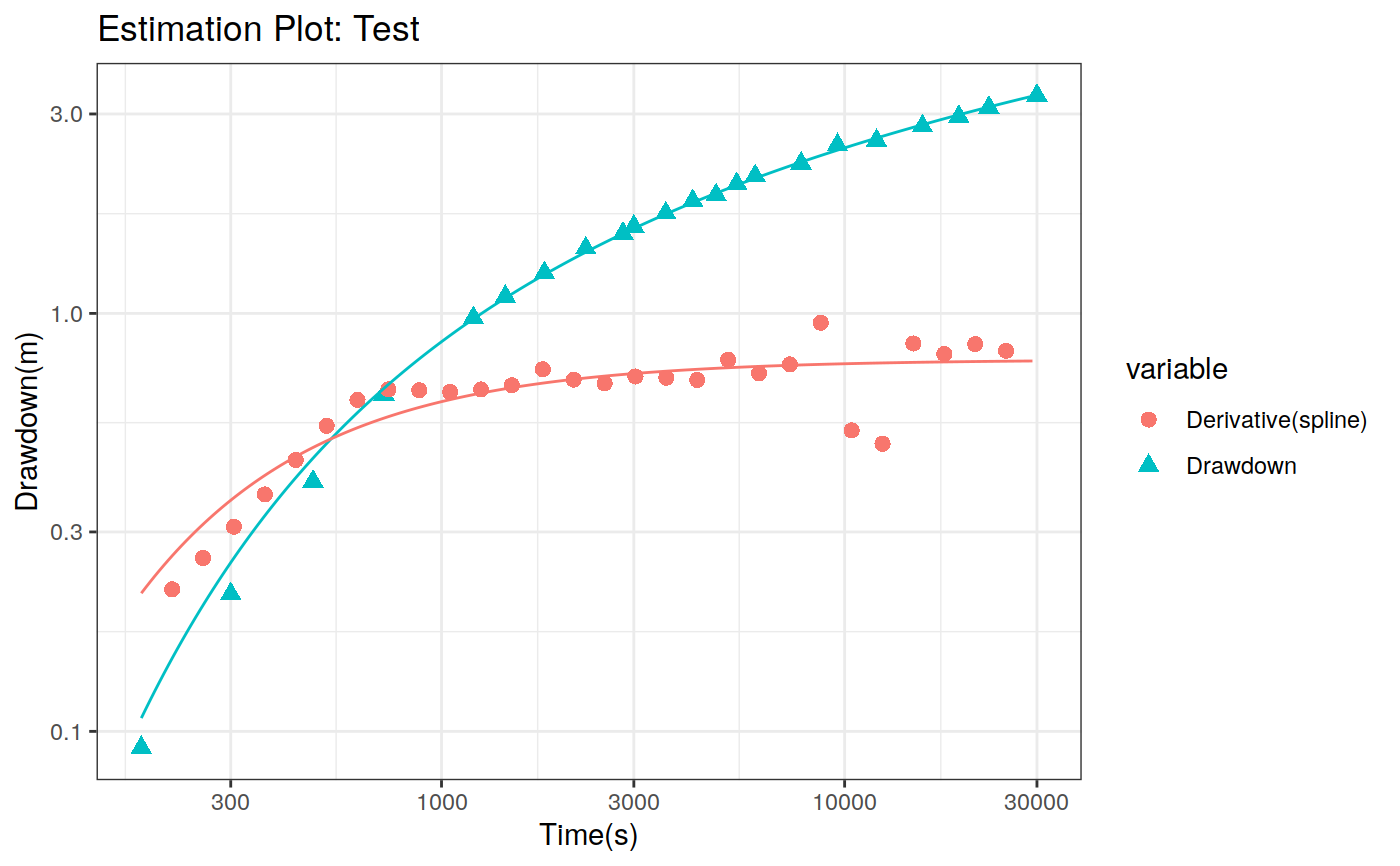
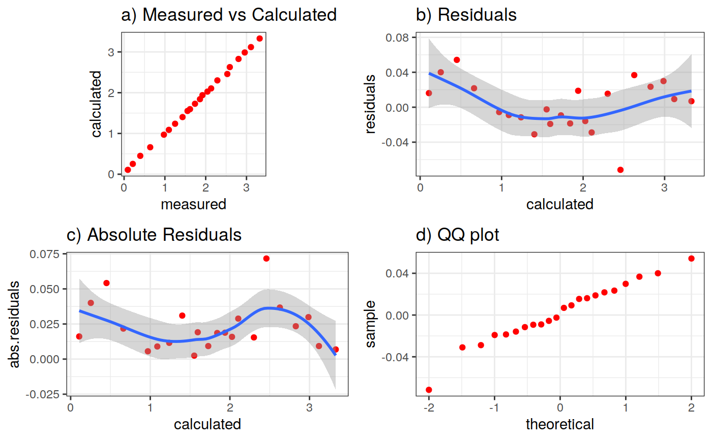
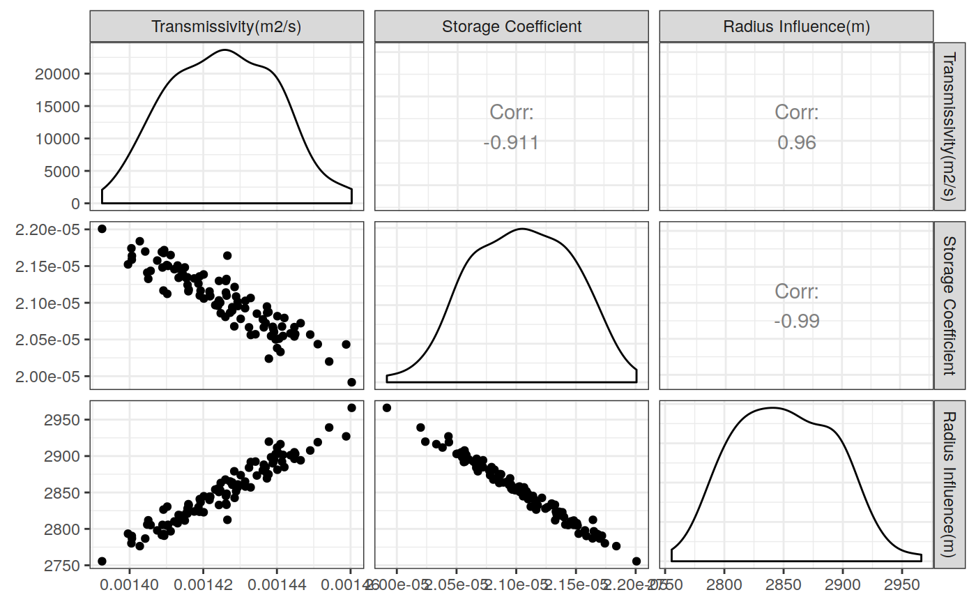
# Define a pumping test
data(theis)
ptest <- pumping_test("Test", Q = 1.388e-2, r = 250, t = theis$t, s = theis$s)
# Diagnostic plot using default parameters
plot(ptest)
#> Joining, by = c("t", "s", "variable")
# Diagnostic plot with Horner derivative
plot(ptest, dmethod = 'horner')
#> Joining, by = c("t", "s", "variable")
# Diagnostic plot with Bourdet derivative d = 3
plot(ptest, dmethod = 'bourdet', d = 3)
#> Joining, by = c("t", "s", "variable")
# Diagnostic plot with Spline derivative
plot(ptest, dmethod = 'spline', d = 20)
#> Joining, by = c("t", "s", "variable")
# Diagnostic plot with semilog scale
plot(ptest, scale = 'slog')
#> Joining, by = c("t", "s", "variable")
#estimation Plot
ptest.fit <- fit(ptest, "theis")
hydraulic.parameters(ptest) <- ptest.fit$hydraulic_parameters
fit.parameters(ptest) <- ptest.fit$parameters
model(ptest) <- "theis"
estimated(ptest) <- TRUE
plot(ptest, type = 'estimation', dmethod = "spline", d = 30, results = FALSE)
#> Joining, by = c("t", "s", "variable")
# Model Diagnostic plot
plot(ptest, type = 'model.diagnostic')
#> Joining, by = c("t", "s", "variable")
#> `geom_smooth()` using method = 'loess' and formula 'y ~ x'
#> `geom_smooth()` using method = 'loess' and formula 'y ~ x'
#> TableGrob (2 x 2) "arrange": 4 grobs
#>   z     cells    name           grob
#> 1 1 (1-1,1-1) arrange gtable[layout]
#> 2 2 (1-1,2-2) arrange gtable[layout]
#> 3 3 (2-2,1-1) arrange gtable[layout]
#> 4 4 (2-2,2-2) arrange gtable[layout]
# Uncertainty plot (bootstrap)
ptest.confint <- confint(ptest, level = c(0.025, 0.975), method = 'bootstrap', n = 30, neval = 100)
hydraulic.parameters(ptest) <- ptest.confint$hydraulic.parameters
hydraulic.parameter.names(ptest) <- ptest.confint$hydraulic.parameters.names
plot(ptest, type = 'uncertainty')
#> Joining, by = c("t", "s", "variable")