plot.ves

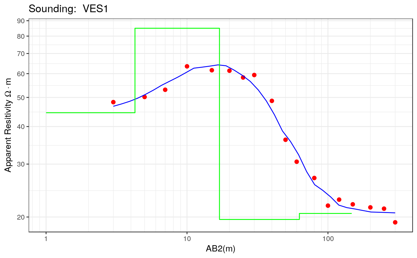
Function to plot the Vertical Electric Sounding data. This function can create two different types of plots: resistivity and interpretation. The resistivity plot includes the apparent resistivity vs electrode spacing. In the interpretation plot, the values of the apparent resistivity vs electrode spacing and the thickness and real resisitivity of the layers are included.

# S3 method for ves
plot(x, main = NULL, type = c("ves", "transformation",
  "diagnostic"), trans.type = c("direct", "scaling", "zohdy",
  "zohdy.smoothed"), ...)

Arguments

x	A VES object
main	Title of the plot
type	A character string specifying the plot type. Currently only ves (measurements and earth model), transformation (resistivity-depth transformation) and diagnostic are supported.
trans.type	A character string specifying the transformation type. Only direct, scaling, zohdy and zohdy.smoothed are currently supported.
...	Additional parameters to be passed to the plot function

See also

Other base functions: print.ves, summary.ves, ves

Examples

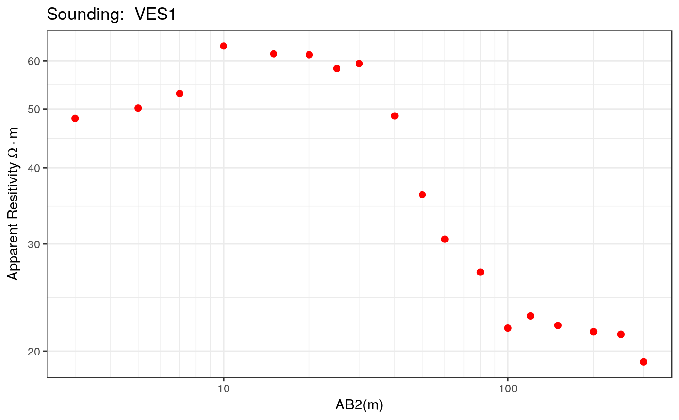
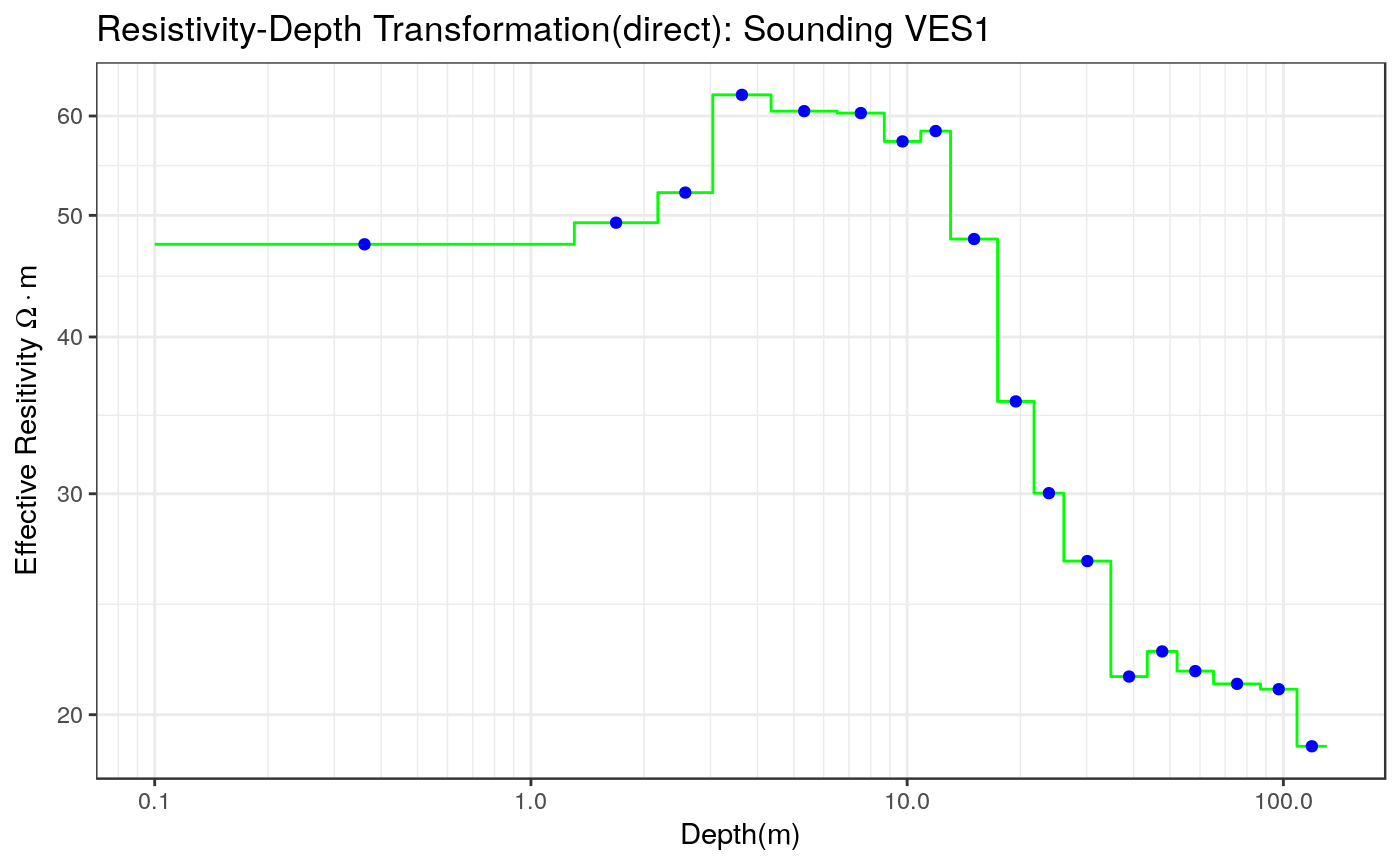
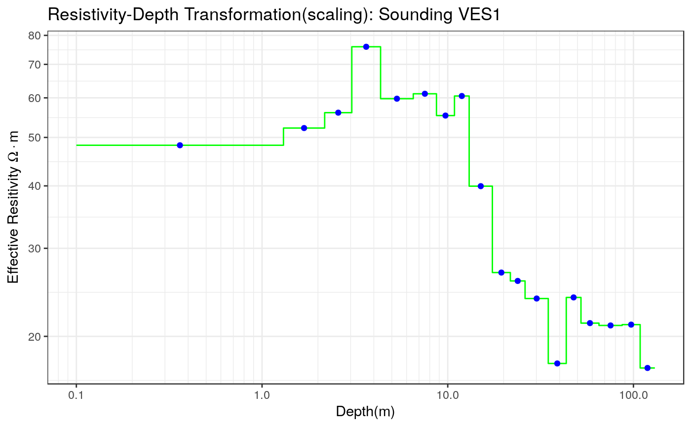
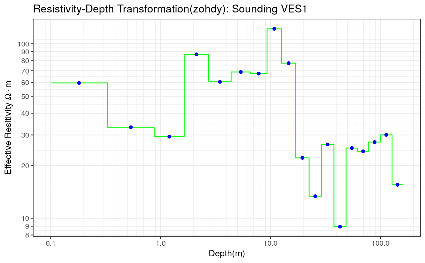
library(grid)
library(gridExtra)
data(ves_data1)
ab2 <- ves_data1$ab2
apprho <- ves_data1$apprho
sev1a <- ves(id= "VES1", ab2 = ab2, apprho = apprho)
# Conventional VES plot
plot(sev1a, type = "ves")
# Apply direct transformation to sev1a
plot(sev1a, type = "transformation", trans.type = "direct")
# Apply scaling transformation to sev1a
plot(sev1a, type = "transformation", trans.type = "scaling")
# Apply Zohdy transformation to sev1a
plot(sev1a, type = "transformation", trans.type = "zohdy")
# Apply Zohdy smoothed transformation to sev1a
plot(sev1a, type = "transformation", trans.type = "scaling")
# Diagnostic plot
rho <- c(40,70,30, 20)
thick <- c(2,10,50,500)
par0 <- c(rho, thick)
res.nls <- calibrate_nls(sev1a, par0, iterations = 30, ireport = 5, trace = FALSE)
sev1a$rhopar <- res.nls$rho
sev1a$thickpar <- res.nls$thickness
sev1a$interpreted <- TRUE
p1 <- plot(sev1a, type = "ves")
print(p1)